Mihcak's denoising filter for 2D images
Motivation
A compressible signal is generally composed by only a few principle components. Keeping only principle components and discarding redundant components are the goal of many compression algorithms. We can think of a compressible signal as the composition of many "similar structures", and there exist cheaper ways to represent them. On the contrary, noise is not compressible as it contain only "random structures".
The target of this post is not about compression, but about a denoising algorithm for 2D images as this algorithm shares the same motivation as compression. Both of them aim to identifying random structures in a signal and attempt to remove them.
Wavelet decomposition
Principle components in a natural image are mostly contained in low-frequency band, which are visible to human eyes. Therefore, compression or denoising is usually done on frequency domain. Discrete Fourier Transform is famous for analyzing frequency components of an image. However, it doesn't present the spectrum at different portions or different scales. Wavelet decomposition does.
Going deep into wavelet decomposition stays beyond this post. In the view of linear algebra, if a signal $f(t)$ is on the space spanned by a basis $\Phi(k)$, it can be expressed by linear combination of the basis. $$f(t) = \sum_{k=1}^N a_k \Phi_k(t), \quad k \; \text{is the integer index} \tag{1} \label{1}$$ If the set of $\{\Phi_k\}$ is carefully chosen, there exist another set of $\{\tilde{\Phi}_k\}$ such that they are orthonormal: $$\langle \Phi_i(t), \tilde{\Phi}_j(t)\rangle = \int \Phi_i(t) \tilde{\Phi}^*_j(t) dt = \begin{cases} \delta_{ij} \quad &\text{if } i=j \\ 0 \quad &\text{if } i \neq j \end{cases} \tag{2} \label{2}$$ where $^*$ is the complex conjugate and $\delta_{ij}$ is the unit function. The property ($\ref{2}$) allows to compute $a_k = \langle f(t), \tilde{\Phi}_k(t) \rangle$ as the transform, and (\ref{1}) as the inverse transform.
In 2D wavelet decomposition, we have two kinds of basis functions $\Phi(x,y)$ and $\Psi(x,y)$ corresponding to scaling and wavelet functions. Scaling function $\Phi(x,y)$ plays the role of a low-pass filter $h[m,n]$, while wavelet function $\Psi(x,y)$ corresponds to a high-pass filter $g[m,n]$. There is a tied relation between the set $\{\Phi(x,y), \Psi(x,y)\}$ and $\{g[m,n], h[m,n]\}$. Instead of computing the transform by using $\Phi(x,y)$ and $\Psi(x,y)$, the same result can be obtained by resorting to filtering process with $h[m,n]$ and $g[m,n]$.
Suppose the basis functions are ready, the image $I$ is decomposed into four bands for each decomposition level: LL, HL, LH, HH (L: low-pass, H: high-pass). The band LL contains low-frequency components of the image, while HL, LH, HH represent variations along $x$-axis, $y$-axis, and diagonal. One can decide to decompose $I$ with more than one level, where the subsequent level is performed on the current LL band instead of $I$. After one decomposition level, the resolution is halved to haft. Shown in Figure 1 is the level 1 decomposition of 512x512 image of lina. There are 4 corresponding bands, and each is 256x256.
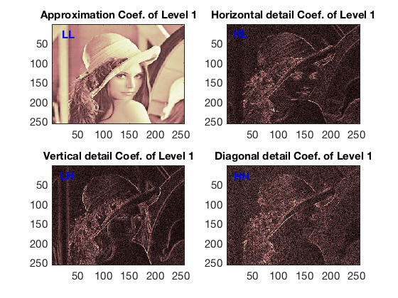
Figure 1. Wavelet decomposition level 1 of lina.
Mihcak’s denoising filter
HL, LH, HH account for high-frequency components including noise, thus denoising will be employed on these three bands. For most of denoising algorithms, the distributions of noise and data have to be made. Mihcak's et al. made assumptions that the noise is Additive White Gaussian Noise (AWGN), and the wavelet coefficients (elements of HL, LH, HH) are independent and identically distributed (i.i.d) Gaussian random variables. Since wavelet coefficients is locally distributed, it is hard to assume a wavelet coefficients as global i.i.d. Therefore, Mihcak et al. relax the assumption so that wavelet coefficients are local i.i.d. With this assumption, Mihcak's filter is designed so that it is capable to adapt itself to different image regions (spatial adaptivity).
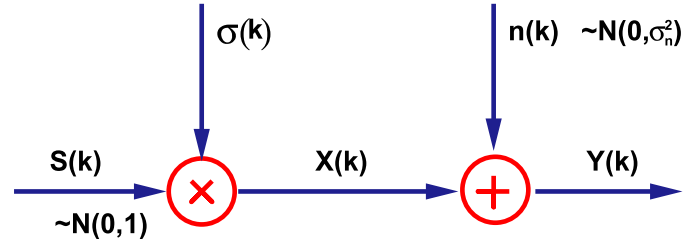
Figure 2. Statistical model. [2]
In statistical model in Figure 2, $x[k]$ is a wavelet coefficient of the clean image, which is a local i.i.d Gaussian random variable, i.e. $x[k] \sim N(0, \sigma(k)^2)$. The observed wavelet coefficient $y[k]$ is essentially $x[k]$ corrupted by AWGN $n[k] \sim N(0,\sigma_n^2)$.
Mihcak's filtering are described in the followings:
Input: $y[k], \sigma_n^2$
Output: the estimate $\hat{x}[k]$
Step 1. Estimate the local variance $\sigma[k]^2$of $x[k]$
The estimation of $\sigma[k]^2$ is done at at $M$ different local neighborhood areas. Let denote $\sigma_m[k]^2$ the variance in the local neighborhood $m$ ($1 \leq m \leq M$). The estimation can be theoretically done by minimizing the mean square error of $\hat{x}[k]$ and $x[k]$.
$$ \underset{\sigma_m[k]}{\min.} \quad \mathbb{E}\left[(\hat{x}[k] - x[k])^2\right]$$ This optimization problem is intractable since we do not have $x[k]$. Based on a reasonable hypothesis that local neighborhoods have similar variance, what we need to choose is a local variance closest to the true one. $$\begin{eqnarray} \hat{\sigma}[k] &=& \underset{\Theta_m}{\text{arg}\min} \quad \mathbb{E}\left[ (\sigma[k] - \Theta_m(k))^2 \right] \\ &=& \underset{\Theta_m}{\text{arg}\min} \quad \left\{ \sigma[k]^2 - 2\sigma[k] \mathbb{E}[\Theta_m[k]] + \mathbb{E}[\Theta_m[k]^2] \right\} \\ &=& \underset{\Theta_m}{\text{arg}\min} \quad \left\{ \sigma[k]^2 - 2\sigma[k] \mathbb{E}[\Theta_m[k]] + \mathbb{E}[]\Theta_m[k]]^2 + \mathbb{Var}[\Theta_m[k]^2] \right\} \\ &=& \underset{\Theta_m}{\text{arg}\min} \quad \left\{ \underbrace{\left(\mathbb{E}[\Theta_m[k]] - \sigma[k] \right)^2}_{\text{term 1}} + \underbrace{\mathbb{Var} \left[ \Theta_m[k]^2 \right]}_{\text{term 2}} \right\} \label{3} \tag{3} \end{eqnarray}$$
This optimization is not solvable if $\sigma[k]$ is involved in. Fortunately, the authors experimentally showed that $\text{term 2}$ dominates $\text{term 1}$ in ($\ref{3}$). Therefore, ($\ref{3}$) is approximated to: $$\hat{\sigma}[k] = \underset{\Theta_m}{\text{arg}\min} \quad \mathbb{Var} \left[ \Theta_m[k]^2 \right]$$
To estimate $\Theta_m^2[k]$ in block $m$, we need to compute the variance $\Theta_m[l]^2$ of every wavelet coefficient $l$ in the block. Given the observation $y[l] = x[l] + n[l]$, the estimate of $\Theta_m[l]^2$ is obtained by maximum log likelihood. $$ \underset{\Theta_m[l]}{\max.} \quad \log \left( \frac{1}{\sqrt{2\pi(\Theta_m[l]^2 + \sigma_n^2)}} \right) - \frac{y[l]}{2(\Theta_m[l]^2 + \sigma_n^2)} \label{4} \tag{4} $$
Solving (\ref{4}), we get the closed-form solution $\Theta_m[l]^2 = y[l]^2 - \sigma_n^2$ and $\Theta_m[l]^2 \neq 0$. After that, $\Theta_m[k]^2$ is estimated as the non-negative mean of $\Theta_m[l]^2$. $$\Theta_m[k]^2 = \max \left\{ 0, \frac{1}{\left|\mathcal{N}_{km} \right|}\underset{l \in \mathcal{N}_{km}}{\sum} y[l]^2 - \sigma_n^2 \right \}, \quad \mathcal{N}_{km} \text{ is the neighborhood } m \text{ of coefficient } k. $$ Now we have $\Theta_m[k]^2$ at block $m$, we next evaluate our estimator $\Theta_m[k]^2$ by computing its variance. This is done by a simple method called bootstrapping. The idea is to resample local neighborhood $m$ with replacement (choosing randomly and independently many local areas $m'$ such that $\left | \mathcal{N}_{km'} \right | = \left | \mathcal{N}_{km} \right |$ ) and estimate $\Theta_{m'}[k]^2$. The variance $\mathbb{Var}(\Theta_m[k]^2)$ can be computed from our population. Finally, $\Theta_m[k]^2$ that has minimal variance is a good estimate of $\hat{\sigma}[k]^2$.
Step 2. Estimate $\hat{x}[k]$. Estimating $\hat{x}[k]$ is equivalent to computing conditional expectation $\hat{x}[k] = \mathbb{E}(x[k] | y[k])$. This computation is very difficult if we don't make further assumption about the class of the estimator. Here the estimator is assumed to be linear: $$\hat{x}[k] = wy[k] + b$$
We need to find $w$ and $b$ minimizing mean square error. This estimation method is referred to as Linear Minimum Mean Square Error (LMMSE). The optimal estimator has to satisfy two conditions:
- The estimator is unbiased. This means $$\begin{eqnarray} \mathbb{E}[\hat{x}[k]] &=& \mathbb{E}[x[k]] \\ w\mathbb{E}[y[k]] + b &=& \mathbb{E}[x[k]] = 0 \\ \text{then } b &=& 0 \end{eqnarray}$$
- The estimation error is minimum. In Figure 3, the estimation error is minimum when it is orthogonal to $y[k]$. For univariate case, this means $$\begin{eqnarray} \mathbb{E}[(\hat{x}[k] - x[k])y[k]] &=& 0 \\ \mathbb{E}[(wy[k] - x[k])y[k]] &=& 0 \\ w\mathbb{E}[y[k]^2] - \mathbb{E}[x[k](x[k] + n[k])] &=& 0 \\ w &=& \frac{\mathbb{E}[x[k]^2] + \mathbb{E}[x[k]]\mathbb{E}[n[k]]}{E[y[k]^2]} \\ w &=& \frac{\mathbb{Var}(x[k])}{\mathbb{Var}(y[k])} = \frac{\sigma[k]^2}{\sigma[k]^2 + \sigma_n^2} \end{eqnarray}$$
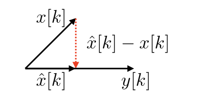
Figure 3. Illustration of LMMSE estimator.
However, we do not have the true $\sigma[k]^2$, but only its estimate $\hat{\sigma}[k]^2$ in Step 1. Finally, $$ \hat{x}[k] = \frac{\hat{\sigma}[k]^2}{\hat{\sigma}[k]^2 + \sigma_n^2} y[k] $$
Once all wavelet coefficients $\hat{x}[k]$ of LH,HL,HH are estimated, we can apply inverse wavelet transform to obtain the clean image. Please refer to Figure 4 for an illustration, where Mihcak filter is applied on the first decomposition level of Lena image.
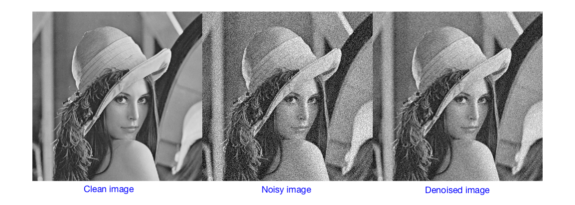
Figure 4. Lena example.
References
- Chun-Lin, Liu, A Tutorial of the Wavelet Transform. 2010.
- M. K. Mihcak, I. Kozintsev, K. Ramchandran, Spatially adaptive statistical modeling of wavelet image coefficients and its application to denoising. 1999.
I am Quoc Tin Phan, the 3rd-year PhD student of the University of Trento, Italy. My research interest is multimedia forensics and applied machine learning.
quoctin.phan@unitn.it